2  Generalized linear mixed models

Notes are adapted from here.

Packages you may need for this lesson:

library(ggplot2)
Warning: package 'ggplot2' was built under R version 4.2.3
library(GGally)
Warning: package 'GGally' was built under R version 4.2.3
Registered S3 method overwritten by 'GGally':
  method from   
  +.gg   ggplot2
library(reshape2)
library(lme4)
Loading required package: Matrix
Warning: package 'Matrix' was built under R version 4.2.3
library(compiler)
library(parallel)
library(boot)
Warning: package 'boot' was built under R version 4.2.2
library(tidyverse)
Warning: package 'tidyverse' was built under R version 4.2.1
── Attaching packages
───────────────────────────────────────
tidyverse 1.3.2 ──
✔ tibble  3.2.1     ✔ dplyr   1.1.4
✔ tidyr   1.3.1     ✔ stringr 1.5.1
✔ readr   2.1.2     ✔ forcats 0.5.2
✔ purrr   1.0.2     
Warning: package 'tibble' was built under R version 4.2.3
Warning: package 'tidyr' was built under R version 4.2.3
Warning: package 'readr' was built under R version 4.2.1
Warning: package 'purrr' was built under R version 4.2.3
Warning: package 'dplyr' was built under R version 4.2.3
Warning: package 'stringr' was built under R version 4.2.3
Warning: package 'forcats' was built under R version 4.2.1
── Conflicts ────────────────────────────────────────── tidyverse_conflicts() ──
✖ tidyr::expand() masks Matrix::expand()
✖ dplyr::filter() masks stats::filter()
✖ dplyr::lag()    masks stats::lag()
✖ tidyr::pack()   masks Matrix::pack()
✖ tidyr::unpack() masks Matrix::unpack()
library(lattice)

Attaching package: 'lattice'

The following object is masked from 'package:boot':

    melanoma

2.1 Methodology overview

2.1.1 Model structure

Here, we briefly cover generalized linear mixed models (GLMMs). GLMMs should be used when you have clustered data, and a response variable that is not continuous. They can mainly be fit with the glmm package in R. package in R. You may need other packages for multinomial (mclogit) and cumulative logit (clmm) regression. In general, the GLMM is the child of LMMs and GLMs. Link functions and random effects join forces!

We may consider the linear predictor: \[\eta=X\alpha+Z\beta.\] The link function allows us to LINK the response \(Y\) to \(\eta\). We can then define:

  • \(\eta=X\alpha+Z\beta\)
  • \(g\) – the link function
  • \(g^{-1}\) – the inverse link function

We can the concisely write our model as: \(g(E(Y))=\eta\), \(E(Y)=g^{-1}(\eta)\) and \(Y=g^{-1}(\eta)+\epsilon\).

For instance, popular link functions include:

  • logit: \(g(x)=logit(x)=\log(x/(1-x))\) – for binary response
  • log: \(g(x)=\log(x)\) – for count response
  • identity: \(g(x)=x\) – continuous

2.1.2 Interpretations

  • The interpretations at the population level follow that of usual GLMs/mixed models. For instance, in logistic mixed regression, you may talk about the probability of a success for different levels of predictors. Or you might say an increase in a predictor causes a certain change in the log odds of a success.

For example, you may wish to recall that:

  • \(logit(P(A))=\log(odds(A))=\log(P(A)/(1-P(A)))\) is the log odds of \(A\) happening.
  • \(odds(A)/odds(B)\) is the odds ratio of \(A\) to \(B\)
  • \(P(A)/P(B)\) is the relative risk of \(A\) to \(B\)

For instance, we may consider \(OR=odds(male\ gets\ disease)/odds(female\ gets\ disease)\). In the logistic model, we have that \(\log(odds(male\ gets\ disease)/odds(female\ gets\ disease))=\alpha_{gender}\). The usual interpretation is holding all other variables fixed, in the case of a GLMM, this includes the random effect. Then, \(\alpha_{gender}\) would be the increase in log odds for someone in the same cluster.

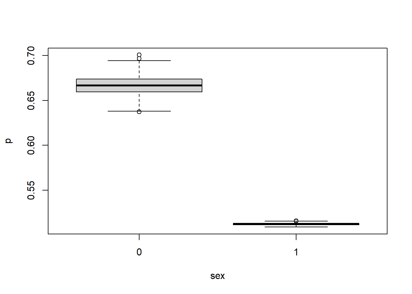
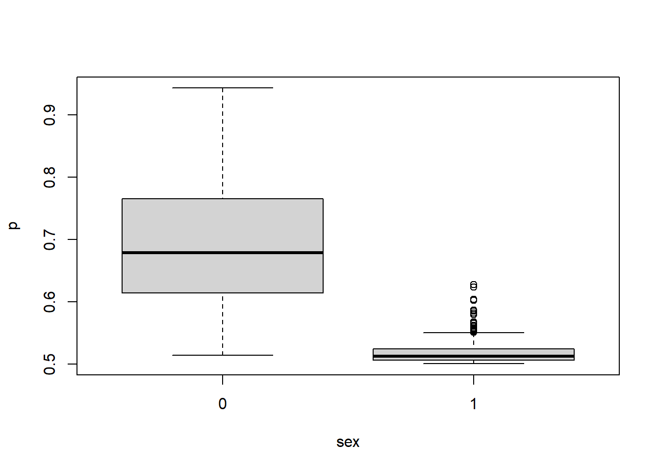
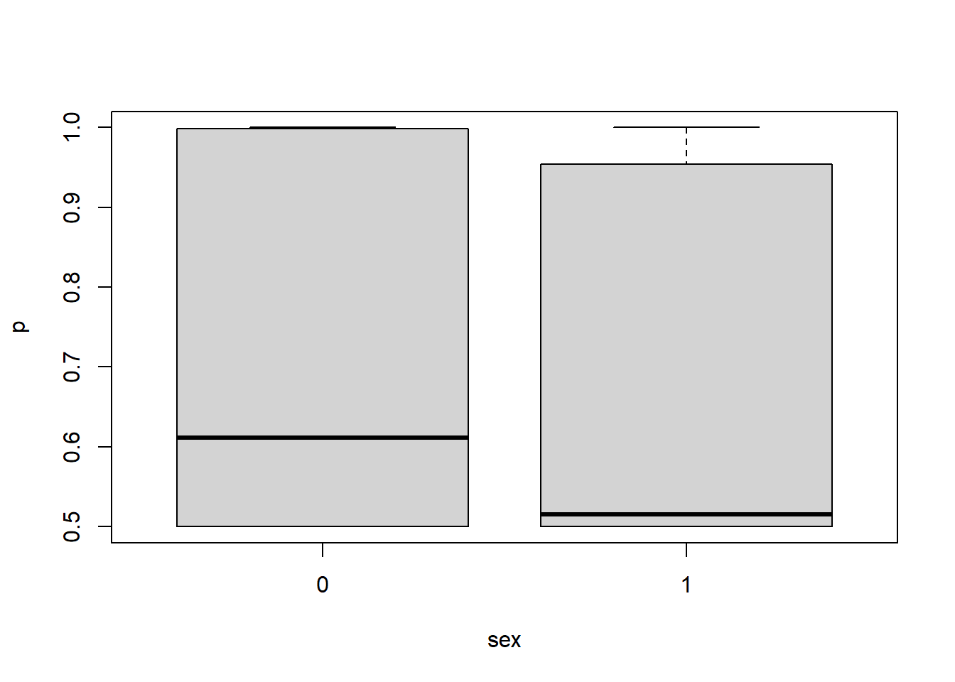
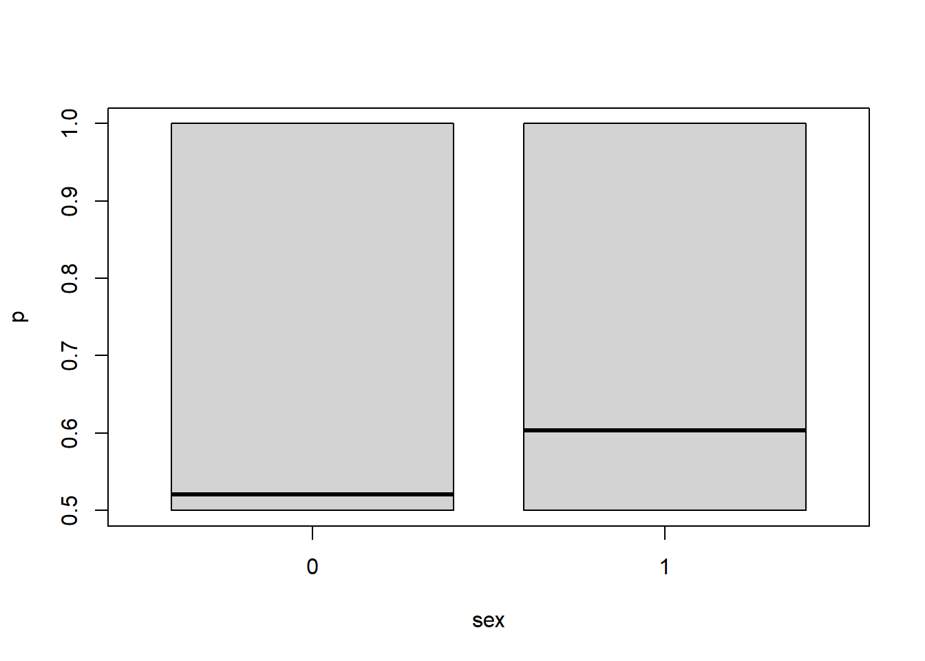
If there is large variability between clusters, the fixed effects may be comparatively small. It is important to see the effect on the probability. Let’s see the impact of different levels of variability on the probability of, say recovery, based off of sex:

expit=function(x){(1+exp(-x))}
simulate_p=function(re_var=1,n=1000){

  
  sex=rbinom(n,1,1/2)
  re=rnorm(n,0,re_var)
  alpha=3
  odds=expit(sex*alpha+re)
  p=odds/(1+odds)
  boxplot(p~sex)
}
simulate_p(0.1)

simulate_p(1)

simulate_p(10)

simulate_p(25)

We can do something similar for count data. If we consider a Poisson model, with the log link, we have that

simulate_count=function(re_var=1,n=1000){

  
  sex=rbinom(n,1,1/2)
  re=rnorm(n,0,re_var)
  alpha=log(5)
  EX_Count=exp(log(10)+re+sex*alpha)
  boxplot(EX_Count~sex)
}
simulate_count(0.1)

simulate_count(0.5)

simulate_count(1)

simulate_count(2)

2.1.3 Final notes

  • The estimates are usually computed via QMLE, or MCMC methods
  • Can take long to fit them
  • Need enough samples at each level

2.2 Case study 2.1

In general, you will have to learn about specific GLMMs individually/case-by-case, so we will proceed with a case study. The following is adapted from: here .

Case information: What patient and physician factors explain lung cancer remission after treatment?

Setup:

hdp = read.csv("https://stats.idre.ucla.edu/stat/data/hdp.csv")
hdp = within(hdp, {
  Married = factor(Married, levels = 0:1, labels = c("no", "yes"))
  DID = factor(DID)
  HID = factor(HID)
  CancerStage = factor(CancerStage)
})

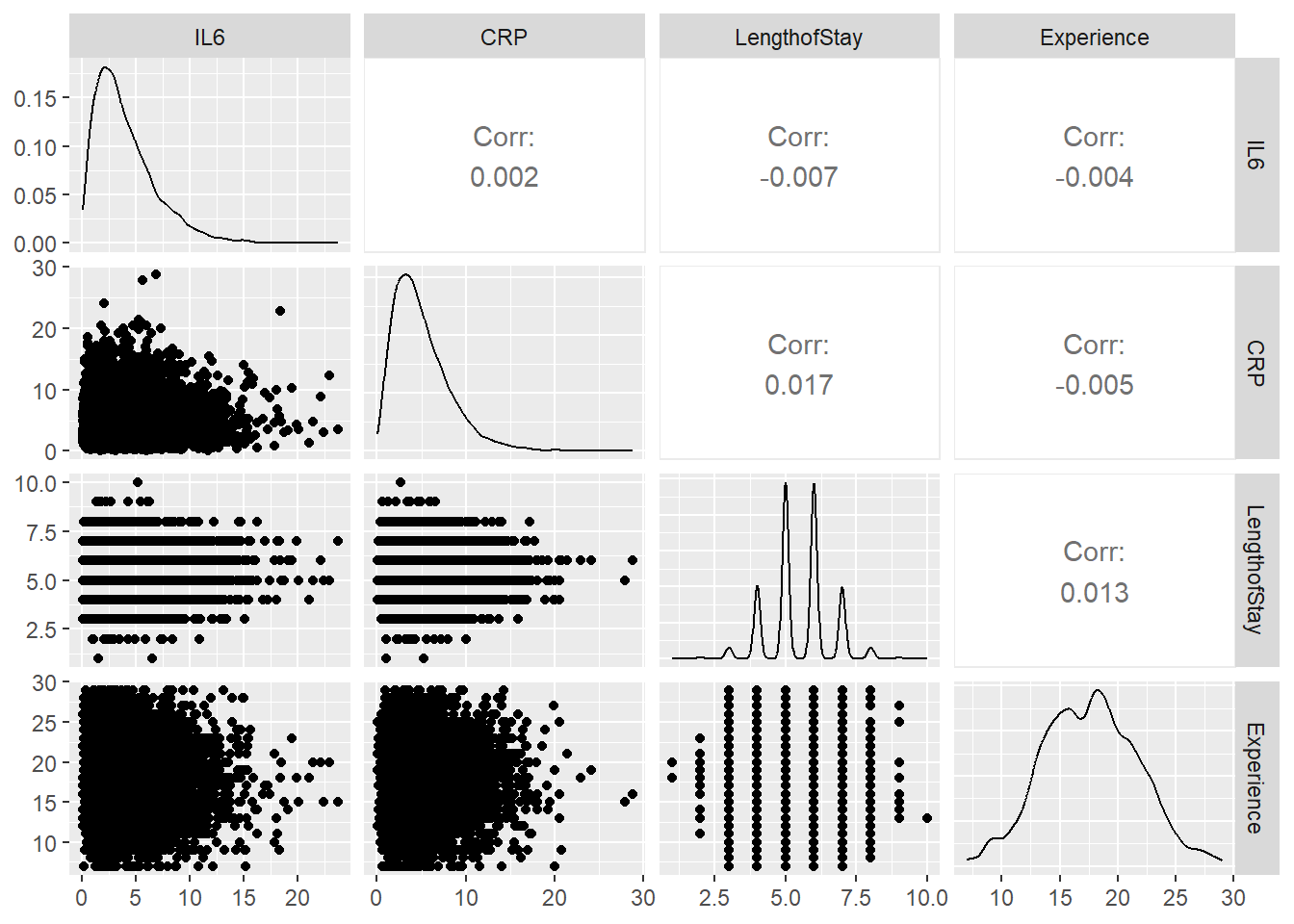
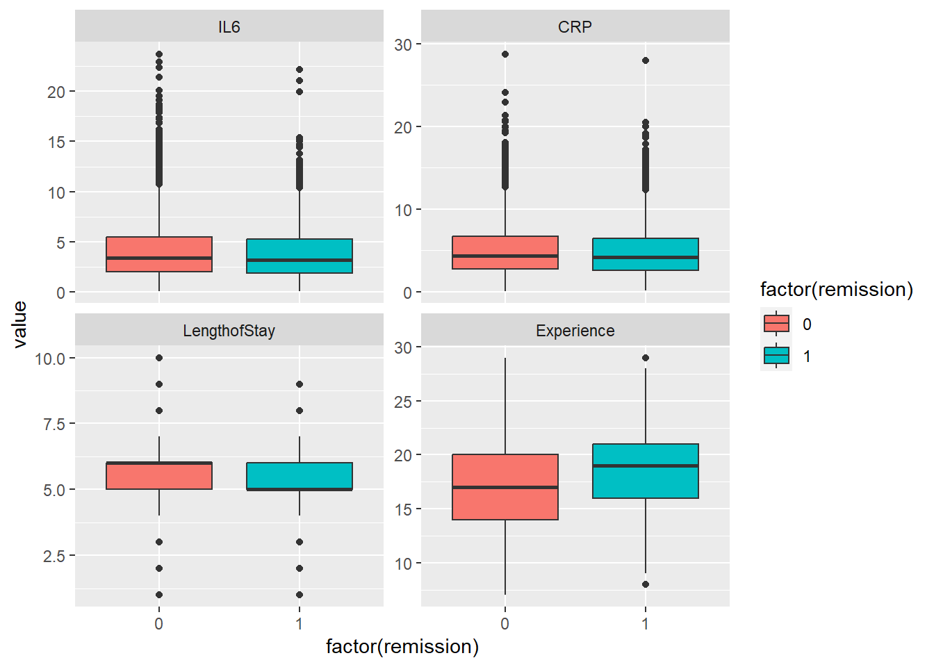
Let’s explore the data, focusing on :

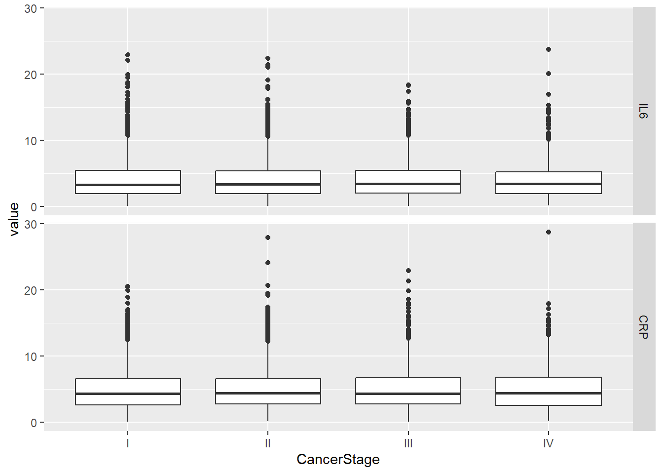
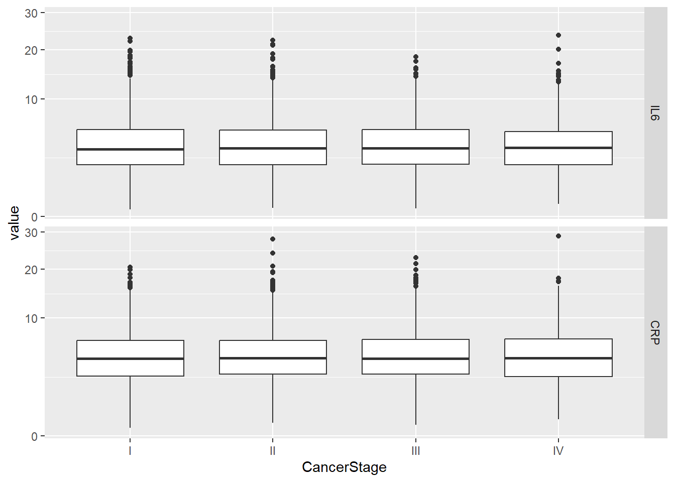
  • Il6, CRP: Biological measurements
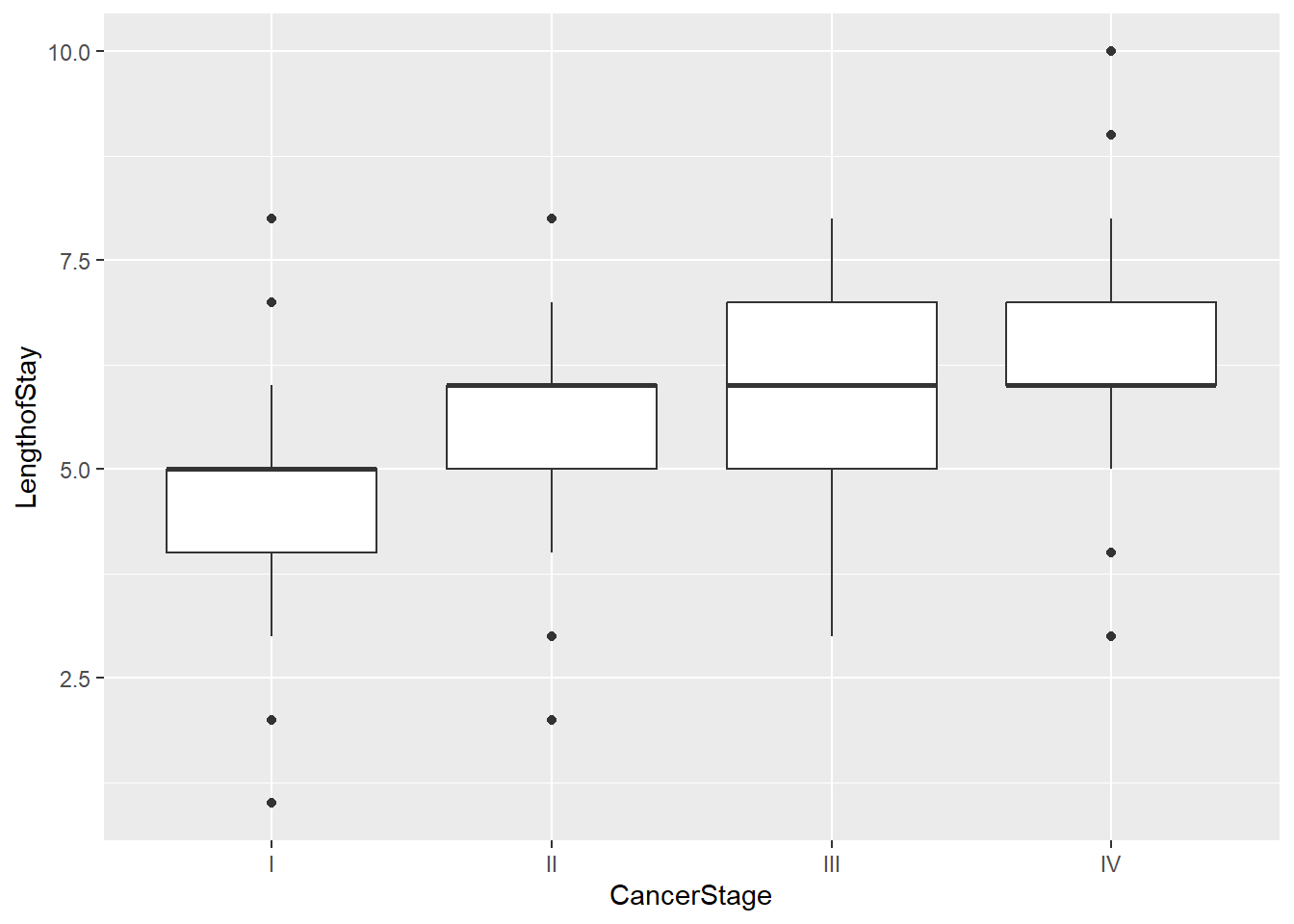
  • LengthofStay
  • CancerStage (I, II, III, or IV),
  • Experience (doctor)
  • doctor ID - cluster variable
head(hdp)
  tumorsize      co2 pain wound mobility ntumors nmorphine remission
1  67.98120 1.534333    4     4        2       0         0         0
2  64.70246 1.676132    2     3        2       0         0         0
3  51.56700 1.533445    6     3        2       0         0         0
4  86.43799 1.453300    3     3        2       0         0         0
5  53.40018 1.566348    3     4        2       0         0         0
6  51.65727 1.417868    4     5        2       0         0         0
  lungcapacity      Age Married FamilyHx SmokingHx    Sex CancerStage
1    0.8010882 64.96824      no       no    former   male          II
2    0.3264440 53.91714      no       no    former female          II
3    0.5650309 53.34730     yes       no     never female          II
4    0.8484109 41.36804      no       no    former   male           I
5    0.8864910 46.80042      no       no     never   male          II
6    0.7010307 51.92936     yes       no     never   male           I
  LengthofStay      WBC      RBC      BMI       IL6       CRP DID Experience
1            6 6087.649 4.868416 24.14424  3.698981 8.0864168   1         25
2            6 6700.310 4.679052 29.40516  2.627481 0.8034876   1         25
3            5 6042.809 5.005862 29.48259 13.896153 4.0341565   1         25
4            5 7162.697 5.265058 21.55726  3.008033 2.1258629   1         25
5            6 6443.440 4.984259 29.81519  3.890698 1.3493239   1         25
6            5 6800.549 5.199714 27.10252  1.418219 2.1946941   1         25
   School Lawsuits HID  Medicaid
1 average        3   1 0.6058667
2 average        3   1 0.6058667
3 average        3   1 0.6058667
4 average        3   1 0.6058667
5 average        3   1 0.6058667
6 average        3   1 0.6058667
names(hdp)
 [1] "tumorsize"    "co2"          "pain"         "wound"        "mobility"    
 [6] "ntumors"      "nmorphine"    "remission"    "lungcapacity" "Age"         
[11] "Married"      "FamilyHx"     "SmokingHx"    "Sex"          "CancerStage" 
[16] "LengthofStay" "WBC"          "RBC"          "BMI"          "IL6"         
[21] "CRP"          "DID"          "Experience"   "School"       "Lawsuits"    
[26] "HID"          "Medicaid"    
# We can use ggplot2 for this one... 
# This si
ggpairs(hdp[, c("IL6", "CRP", "LengthofStay", "Experience")])

ggplot(hdp, aes(x = CancerStage, y = LengthofStay)) +
  geom_boxplot()

tmp = melt(hdp[, c("CancerStage", "IL6", "CRP")], id.vars="CancerStage")
ggplot(tmp, aes(x = CancerStage, y = value)) +
  geom_boxplot() +
  facet_grid(variable ~ .) 

ggplot(tmp, aes(x = CancerStage, y = value)) +
  geom_boxplot() +
  facet_grid(variable ~ .) +
  scale_y_sqrt()

tmp = melt(hdp[, c("remission", "IL6", "CRP", "LengthofStay", "Experience")],
  id.vars="remission")
ggplot(tmp, aes(factor(remission), y = value, fill=factor(remission))) +
  geom_boxplot() +
  facet_wrap(~variable, scales="free_y")

2.2.1 Fitting the model

# mixed effects logistic regression model
# estimate the model
# model = glmer(remission ~ IL6 + CRP + CancerStage + LengthofStay + Experience +
    # (1 | DID), data = hdp, family = binomial)

model = glmer(remission ~ IL6 + CRP + CancerStage + LengthofStay + Experience +
    (1 | DID), data = hdp, family = binomial, control = glmerControl(optimizer = "bobyqa"),nAGQ = 10)
# print the mod results without correlations among fixed effects
print(model, corr = FALSE)
Generalized linear mixed model fit by maximum likelihood (Adaptive
  Gauss-Hermite Quadrature, nAGQ = 10) [glmerMod]
 Family: binomial  ( logit )
Formula: remission ~ IL6 + CRP + CancerStage + LengthofStay + Experience +  
    (1 | DID)
   Data: hdp
      AIC       BIC    logLik  deviance  df.resid 
 7397.276  7460.733 -3689.638  7379.276      8516 
Random effects:
 Groups Name        Std.Dev.
 DID    (Intercept) 2.015   
Number of obs: 8525, groups:  DID, 407
Fixed Effects:
   (Intercept)             IL6             CRP   CancerStageII  CancerStageIII  
      -2.05269        -0.05677        -0.02148        -0.41393        -1.00346  
 CancerStageIV    LengthofStay      Experience  
      -2.33704        -0.12118         0.12009  
# broom::tidy(model)
se = sqrt(diag(vcov(model)))
# table of estimates with 95% CI
tab = cbind(Est = fixef(model), LL = fixef(model) - 1.96 * se, UL = fixef(model) + 1.96 *se); tab
                       Est          LL           UL
(Intercept)    -2.05269401 -3.09430566 -1.011082369
IL6            -0.05677185 -0.07934786 -0.034195848
CRP            -0.02148294 -0.04151100 -0.001454893
CancerStageII  -0.41393409 -0.56243123 -0.265436940
CancerStageIII -1.00346486 -1.19609923 -0.810830493
CancerStageIV  -2.33703717 -2.64682992 -2.027244418
LengthofStay   -0.12118214 -0.18710336 -0.055260913
Experience      0.12008835  0.06628404  0.173892667
#Odds ratios
exp(tab)
                      Est         LL        UL
(Intercept)    0.12838856 0.04530646 0.3638250
IL6            0.94480960 0.92371854 0.9663822
CRP            0.97874617 0.95933879 0.9985462
CancerStageII  0.66104452 0.56982201 0.7668708
CancerStageIII 0.36660700 0.30237140 0.4444888
CancerStageIV  0.09661346 0.07087554 0.1316979
LengthofStay   0.88587259 0.82935801 0.9462382
Experience     1.12759647 1.06853018 1.1899278

Inference - use normal approximation, or bootstrapping… For boostrapping, we need to sample one level at a time.

#resamples single level clustered data
sampler = function(dat, clustervar, replace = TRUE, reps = 1) {
    # Unique clusters
    cid = unique(dat[, clustervar[1]])
    # num clusters
    ncid = length(cid)
    # sampled clusters for each rep
    recid = sample(cid, size = ncid * reps, replace = TRUE)
    if (replace) {
      # This line is grabbing all the rows corresponding to each cluster, sampling them, and assigning a new id
        rid = lapply(seq_along(recid), function(i) {
            cbind(NewID = i, RowID = sample(which(dat[, clustervar] == recid[i]),
                size = length(which(dat[, clustervar] == recid[i])), replace = TRUE))
        })
    } 
    
    else {
      # This line is grabbing all the rows corresponding to each cluster and assigning a new id
        rid = lapply(seq_along(recid), function(i) {
            cbind(NewID = i, RowID = which(dat[, clustervar] == recid[i]))
        })
    }
    #put the above info in a dataframe
    dat = as.data.frame(do.call(rbind, rid))
    
    # put the above info in a dataframe, cut divides the above long samples into the replicate samples. include.lowest just includes the left side of the interval, but not the right
    dat$Replicate = cut(dat$NewID, breaks = c(1, ncid * 1:reps), include.lowest = TRUE,labels = FALSE)%>%factor()
    # change to factor
    dat$NewID = factor(dat$NewID)
    return(dat)
}
head(sampler(hdp, "DID", reps = 1))
  NewID RowID Replicate
1     1  4547         1
2     1  4553         1
3     1  4540         1
4     1  4551         1
5     1  4540         1
6     1  4540         1
set.seed(1241)
#sample 100 samples, use more in reality

tmp = sampler(hdp, "DID", reps = 100)
bigdata = cbind(tmp, hdp[tmp$RowID, ])
head(bigdata)
     NewID RowID Replicate tumorsize      co2 pain wound mobility ntumors
1137     1  1137         1  61.60908 1.385558    4     5        5       4
1131     1  1131         1  62.90957 1.489077    3     5        4       1
1158     1  1158         1  61.15147 1.694328    5     6        4       0
1151     1  1151         1  94.27969 1.752081    5     7        5       2
1152     1  1152         1  85.51482 1.532822    3     6        6       6
1148     1  1148         1  73.29905 1.770178    5     6        6       5
     nmorphine remission lungcapacity      Age Married FamilyHx SmokingHx
1137         7         0    0.9750009 55.83614      no       no     never
1131         4         0    0.9268863 51.04217     yes       no     never
1158         0         0    0.6443683 43.13214     yes       no     never
1151         7         0    0.8582457 62.36135     yes       no   current
1152         5         0    0.4208578 61.63105      no      yes     never
1148         4         0    0.9638132 49.00940      no       no   current
        Sex CancerStage LengthofStay      WBC      RBC      BMI       IL6
1137 female          II            6 4967.423 5.412072 29.58874 6.1558399
1131 female          II            6 5605.937 4.793538 23.66554 3.7553295
1158 female           I            5 5483.016 5.040751 28.64414 2.5412189
1151   male           I            5 6337.338 6.064870 30.33128 3.2348010
1152 female          IV            7 4039.674 5.266622 25.28456 0.7059072
1148   male           I            4 5365.597 4.970115 39.41294 0.7627430
            CRP DID Experience  School Lawsuits HID  Medicaid
1137  1.9068986  52         19 average        3   5 0.2188103
1131  0.6346611  52         19 average        3   5 0.2188103
1158  3.7357859  52         19 average        3   5 0.2188103
1151  8.2530591  52         19 average        3   5 0.2188103
1152  4.4492342  52         19 average        3   5 0.2188103
1148 10.7412680  52         19 average        3   5 0.2188103
f = fixef(model); f
   (Intercept)            IL6            CRP  CancerStageII CancerStageIII 
   -2.05269401    -0.05677185    -0.02148294    -0.41393409    -1.00346486 
 CancerStageIV   LengthofStay     Experience 
   -2.33703717    -0.12118214     0.12008835 
r = getME(model, "theta"); r
DID.(Intercept) 
       2.014552 
# Make cluster
cl = makeCluster(10)
clusterExport(cl, c("bigdata", "f", "r"))
a=clusterEvalQ(cl, require(lme4))
myboot = function(i) {
  # fit the mdoel for every bootstrap sample
    object = try(glmer(remission ~ IL6 + CRP + CancerStage + LengthofStay +
        Experience + (1 | NewID), data = bigdata, subset = Replicate == i, family = binomial,
        nAGQ = 1, start = list(fixef = f, theta = r)), silent = TRUE)
    if (class(object) == "try-error")
        return(object)
    c(fixef(object), getME(object, "theta"))
}
start = proc.time()
res = parLapplyLB(cl, X = levels(bigdata$Replicate), fun = myboot)
end = proc.time()
# shut down the cluster
stopCluster(cl)
#Check how many models converge
success = sapply(res, is.numeric)
mean(success)

# combine successful results
bigres = do.call(cbind, res[success])

# calculate 2.5th and 97.5th percentiles for 95% CI
(ci = t(apply(bigres, 1, quantile, probs = c(0.025, 0.975))))

# All results
finaltable = cbind(Est = c(f, r), SE = c(se, NA), BootMean = rowMeans(bigres),ci)
# round and print
round(finaltable, 3)

2.2.2 Predicted probabilities and graphing

We may wish to plot some of the fitted functions/probabilities.

Now we can look at by length of stay:

# temporary data
tmpdat = hdp[, c("IL6", "CRP", "CancerStage", "LengthofStay", "Experience","DID")]

summary(hdp$LengthofStay)
   Min. 1st Qu.  Median    Mean 3rd Qu.    Max. 
  1.000   5.000   5.000   5.492   6.000  10.000 
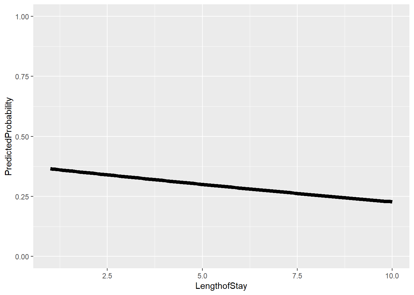
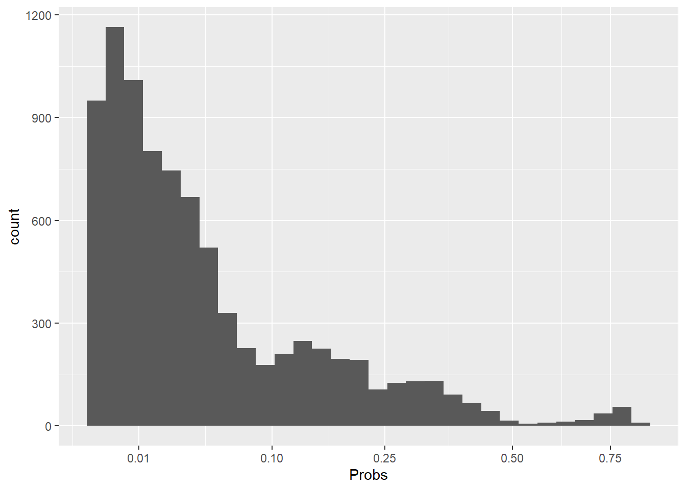
jvalues =  seq(from = min(hdp$LengthofStay), to = max(hdp$LengthofStay), l = 100)

# calculate predicted probabilities and store in a list
pp = lapply(jvalues, function(j) {
    tmpdat$LengthofStay = j
    predict(model, newdata = tmpdat, type = "response")
})

# average marginal predicted probability across a few different Lengths of
# Stay
jvalues[c(1, 20, 40, 60, 80, 100)]
[1]  1.000000  2.727273  4.545455  6.363636  8.181818 10.000000
sapply(pp[c(1, 20, 40, 60, 80, 100)], mean)
[1] 0.3652319 0.3366360 0.3075494 0.2796359 0.2530109 0.2277694
# get the means with lower and upper quartiles
plotdat = t(sapply(pp, function(x) {
    c(M = mean(x), quantile(x, c(0.25, 0.75)))
}))
head(plotdat)
             M        25%       75%
[1,] 0.3652319 0.08489874 0.6155638
[2,] 0.3637056 0.08404676 0.6129535
[3,] 0.3621815 0.08320255 0.6103367
[4,] 0.3606597 0.08236605 0.6077135
[5,] 0.3591402 0.08153722 0.6050841
[6,] 0.3576230 0.08071600 0.6024486
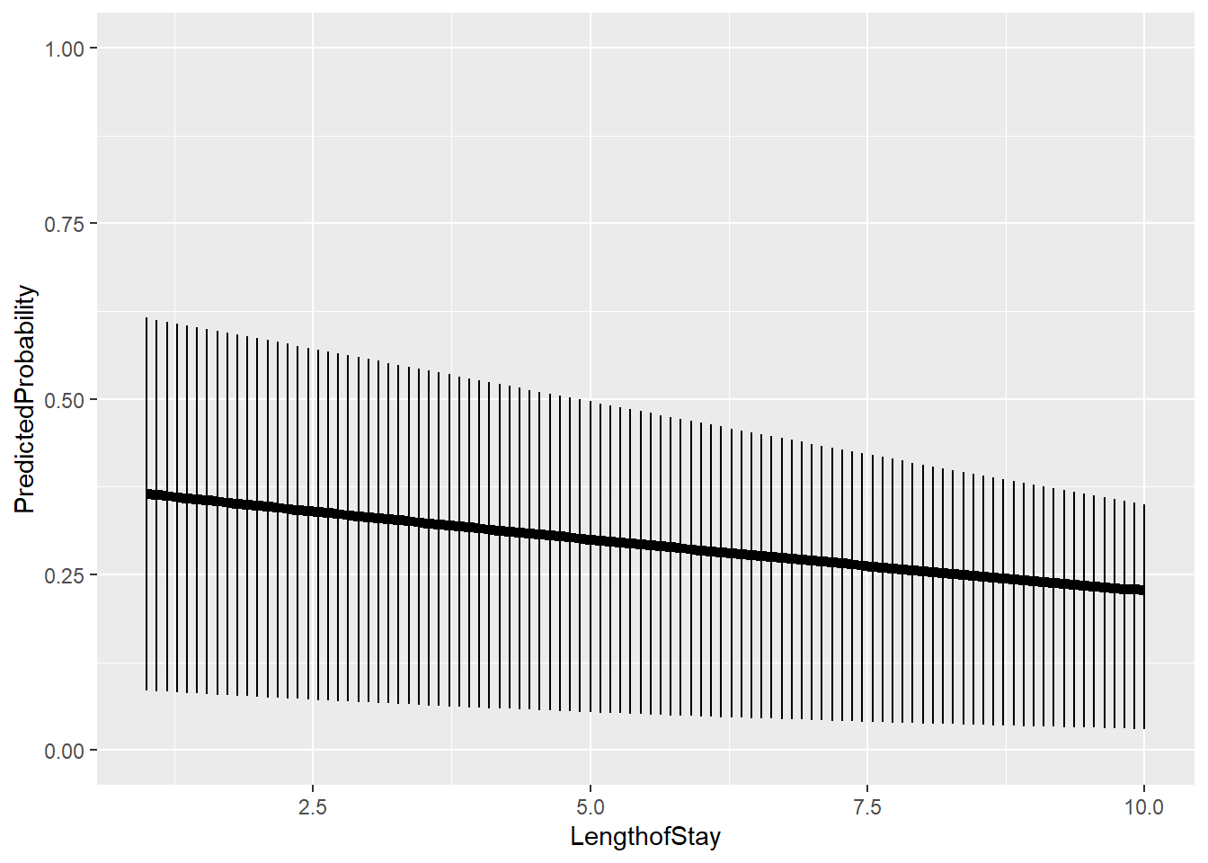
# add in LengthofStay values and convert to data frame
plotdat = as.data.frame(cbind(plotdat, jvalues))

# better names and show the first few rows
colnames(plotdat) = c("PredictedProbability", "Lower", "Upper", "LengthofStay")
head(plotdat)
  PredictedProbability      Lower     Upper LengthofStay
1            0.3652319 0.08489874 0.6155638     1.000000
2            0.3637056 0.08404676 0.6129535     1.090909
3            0.3621815 0.08320255 0.6103367     1.181818
4            0.3606597 0.08236605 0.6077135     1.272727
5            0.3591402 0.08153722 0.6050841     1.363636
6            0.3576230 0.08071600 0.6024486     1.454545
# plot average marginal predicted probabilities
ggplot(plotdat, aes(x = LengthofStay, y = PredictedProbability)) + geom_line(linewidth = 2) +
    ylim(c(0, 1))

ggplot(plotdat, aes(x = LengthofStay, y = PredictedProbability)) + geom_linerange(aes(ymin = Lower,
    ymax = Upper)) + geom_line(linewidth = 2) + ylim(c(0, 1))

#################

Now we can look at by stage:

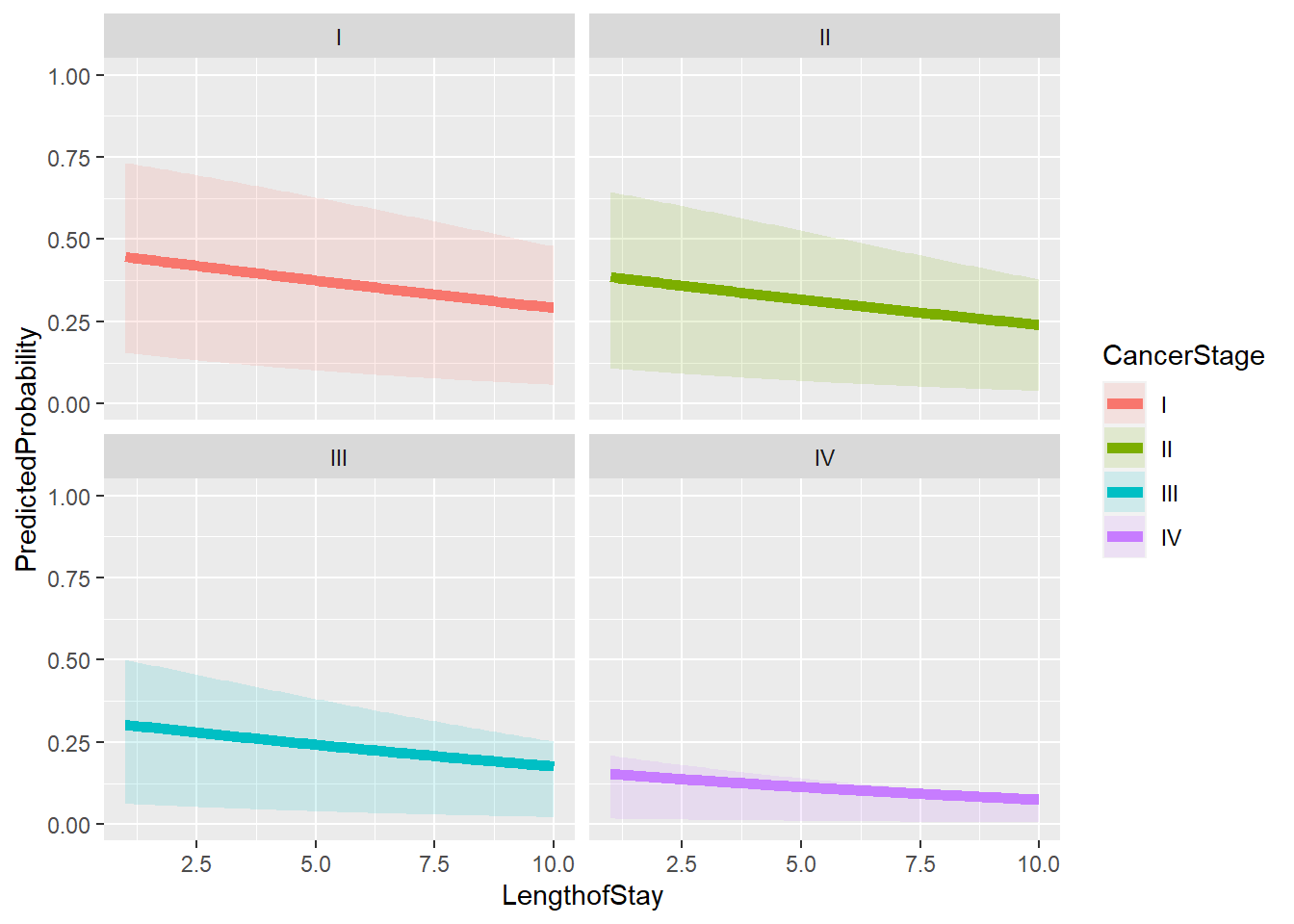
# calculate predicted probabilities for each stage and store in a list
biprobs = lapply(levels(hdp$CancerStage), function(stage) {
  tmpdat$CancerStage = stage
  lapply(jvalues, function(j) {
    tmpdat$LengthofStay = j
    predict(model, newdata = tmpdat, type = "response")
  })
})

# get means and quartiles for all jvalues for each level of CancerStage
plotdat2 = lapply(biprobs, function(X) {
  temp = t(sapply(X, function(x) {
    c(M=mean(x), quantile(x, c(.25, .75)))
  }))
  temp = as.data.frame(cbind(temp, jvalues))
  colnames(temp) = c("PredictedProbability", "Lower", "Upper", "LengthofStay")
  return(temp)
})


# collapse to one data frame
plotdat2 = do.call(rbind, plotdat2)

# add cancer stage
plotdat2$CancerStage = factor(rep(levels(hdp$CancerStage), each = length(jvalues)))

# show first few rows
head(plotdat2)
  PredictedProbability     Lower     Upper LengthofStay CancerStage
1            0.4474662 0.1547407 0.7328360     1.000000           I
2            0.4458001 0.1533052 0.7306736     1.090909           I
3            0.4441352 0.1518807 0.7285001     1.181818           I
4            0.4424716 0.1504671 0.7263157     1.272727           I
5            0.4408092 0.1490643 0.7241204     1.363636           I
6            0.4391481 0.1476723 0.7219142     1.454545           I
# graph it
ggplot(plotdat2, aes(x = LengthofStay, y = PredictedProbability)) +
  geom_ribbon(aes(ymin = Lower, ymax = Upper, fill = CancerStage), alpha = .15) +
  geom_line(aes(colour = CancerStage), size = 2) +
  ylim(c(0, 1)) + facet_wrap(~  CancerStage)
Warning: Using `size` aesthetic for lines was deprecated in ggplot2 3.4.0.
ℹ Please use `linewidth` instead.

ggplot(data.frame(Probs = biprobs[[4]][[100]]), aes(Probs)) + geom_histogram() +
    scale_x_sqrt(breaks = c(0.01, 0.1, 0.25, 0.5, 0.75))
`stat_bin()` using `bins = 30`. Pick better value with `binwidth`.

We may have considered the variation within hospital as well… Or toher variables etc.

# estimate the model and store results in m
m3a = glmer(remission ~ Age + LengthofStay + FamilyHx + IL6 + CRP +
  CancerStage + Experience + (1 | DID) + (1 | HID),
  data = hdp, family = binomial, nAGQ=1)
Warning in checkConv(attr(opt, "derivs"), opt$par, ctrl = control$checkConv, :
Model failed to converge with max|grad| = 0.393634 (tol = 0.002, component 1)
# print the mod results without correlations among fixed effects
print(m3a, corr=FALSE)
Generalized linear mixed model fit by maximum likelihood (Laplace
  Approximation) [glmerMod]
 Family: binomial  ( logit )
Formula: remission ~ Age + LengthofStay + FamilyHx + IL6 + CRP + CancerStage +  
    Experience + (1 | DID) + (1 | HID)
   Data: hdp
      AIC       BIC    logLik  deviance  df.resid 
 7199.081  7283.690 -3587.541  7175.081      8513 
Random effects:
 Groups Name        Std.Dev.
 DID    (Intercept) 1.9513  
 HID    (Intercept) 0.5432  
Number of obs: 8525, groups:  DID, 407; HID, 35
Fixed Effects:
   (Intercept)             Age    LengthofStay     FamilyHxyes             IL6  
      -1.68299        -0.01496        -0.04577        -1.30789        -0.05729  
           CRP   CancerStageII  CancerStageIII   CancerStageIV      Experience  
      -0.02209        -0.31739        -0.85462        -2.13138         0.12703  
optimizer (Nelder_Mead) convergence code: 0 (OK) ; 0 optimizer warnings; 1 lme4 warnings 
hist(ranef(m3a, which = "DID")[[1]][,1])

hist(ranef(m3a, which = "HID")[[1]][,1])

# lattice::dotplot(ranef(m3a, which = "DID", condVar = TRUE), scales = list(y = list(alternating = 0)))
# lattice::dotplot(ranef(m3a, which = "HID", condVar = TRUE))

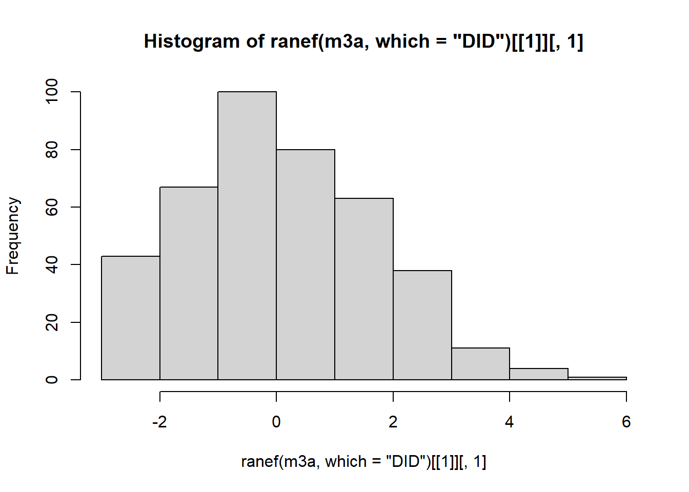
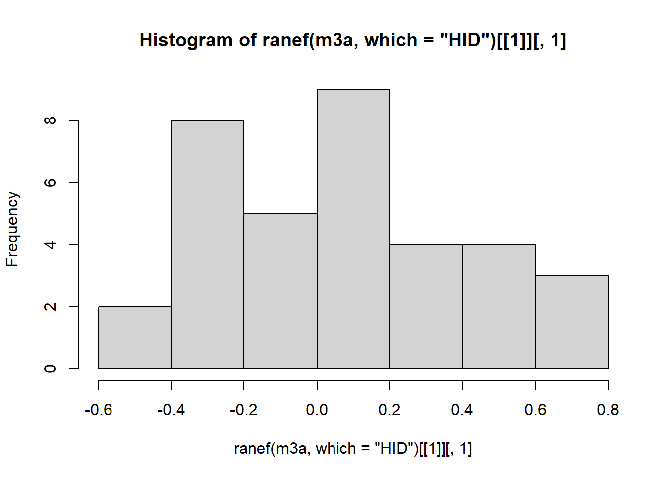
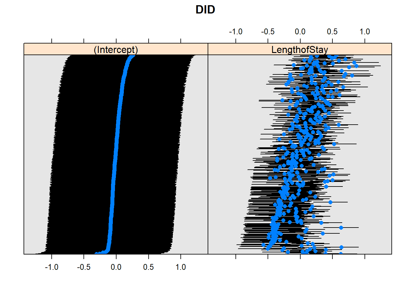
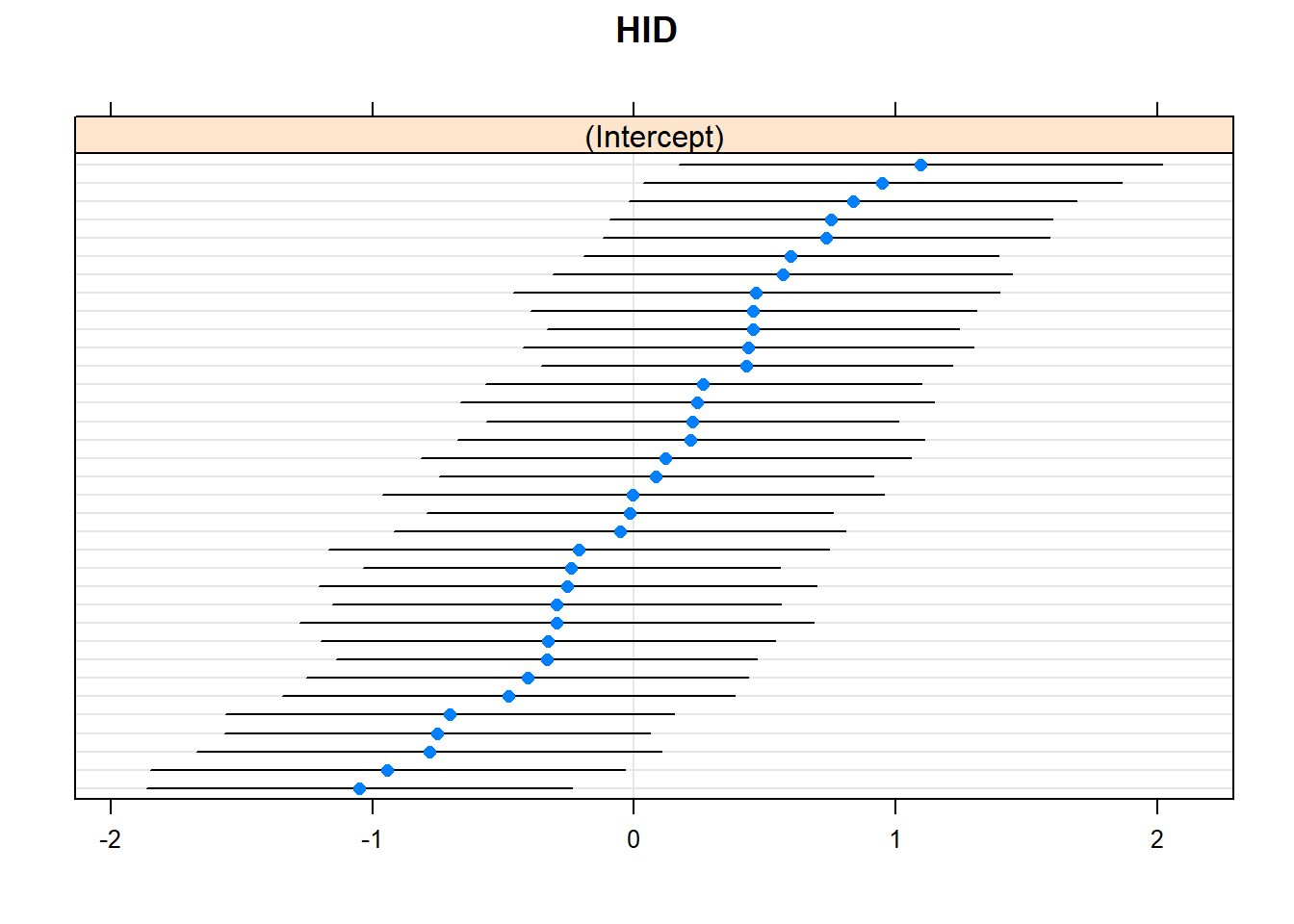
Homework: Try this other model. What is the dotplot saying?

# estimate the model and store results in m
m3b = glmer(remission ~ Age + LengthofStay + FamilyHx + IL6 + CRP + CancerStage +
    Experience + (1 + LengthofStay | DID) + (1 | HID), data = hdp, family = binomial,
    nAGQ = 1)
Warning in checkConv(attr(opt, "derivs"), opt$par, ctrl = control$checkConv, :
Model failed to converge with max|grad| = 1.66877 (tol = 0.002, component 1)
print(m3b, corr = FALSE)
Generalized linear mixed model fit by maximum likelihood (Laplace
  Approximation) [glmerMod]
 Family: binomial  ( logit )
Formula: remission ~ Age + LengthofStay + FamilyHx + IL6 + CRP + CancerStage +  
    Experience + (1 + LengthofStay | DID) + (1 | HID)
   Data: hdp
      AIC       BIC    logLik  deviance  df.resid 
 7147.749  7246.460 -3559.875  7119.749      8511 
Random effects:
 Groups Name         Std.Dev. Corr 
 DID    (Intercept)  0.5029        
        LengthofStay 0.3729   -0.12
 HID    (Intercept)  0.7318        
Number of obs: 8525, groups:  DID, 407; HID, 35
Fixed Effects:
   (Intercept)             Age    LengthofStay     FamilyHxyes             IL6  
      -0.53725        -0.01523        -0.19062        -1.33822        -0.05865  
           CRP   CancerStageII  CancerStageIII   CancerStageIV      Experience  
      -0.02095        -0.29471        -0.86500        -2.30039         0.10412  
optimizer (Nelder_Mead) convergence code: 0 (OK) ; 0 optimizer warnings; 1 lme4 warnings 
lattice::dotplot(ranef(m3b, which = "DID", condVar = TRUE), scales = list(y = list(alternating = 0)))
$DID

lattice::dotplot(ranef(m3b, which = "HID", condVar = TRUE), scales = list(y = list(alternating = 0)))
$HID